The all-in-one platform for private and secure AI
Deploy anywhere — on-prem, private cloud, or fully managed by us
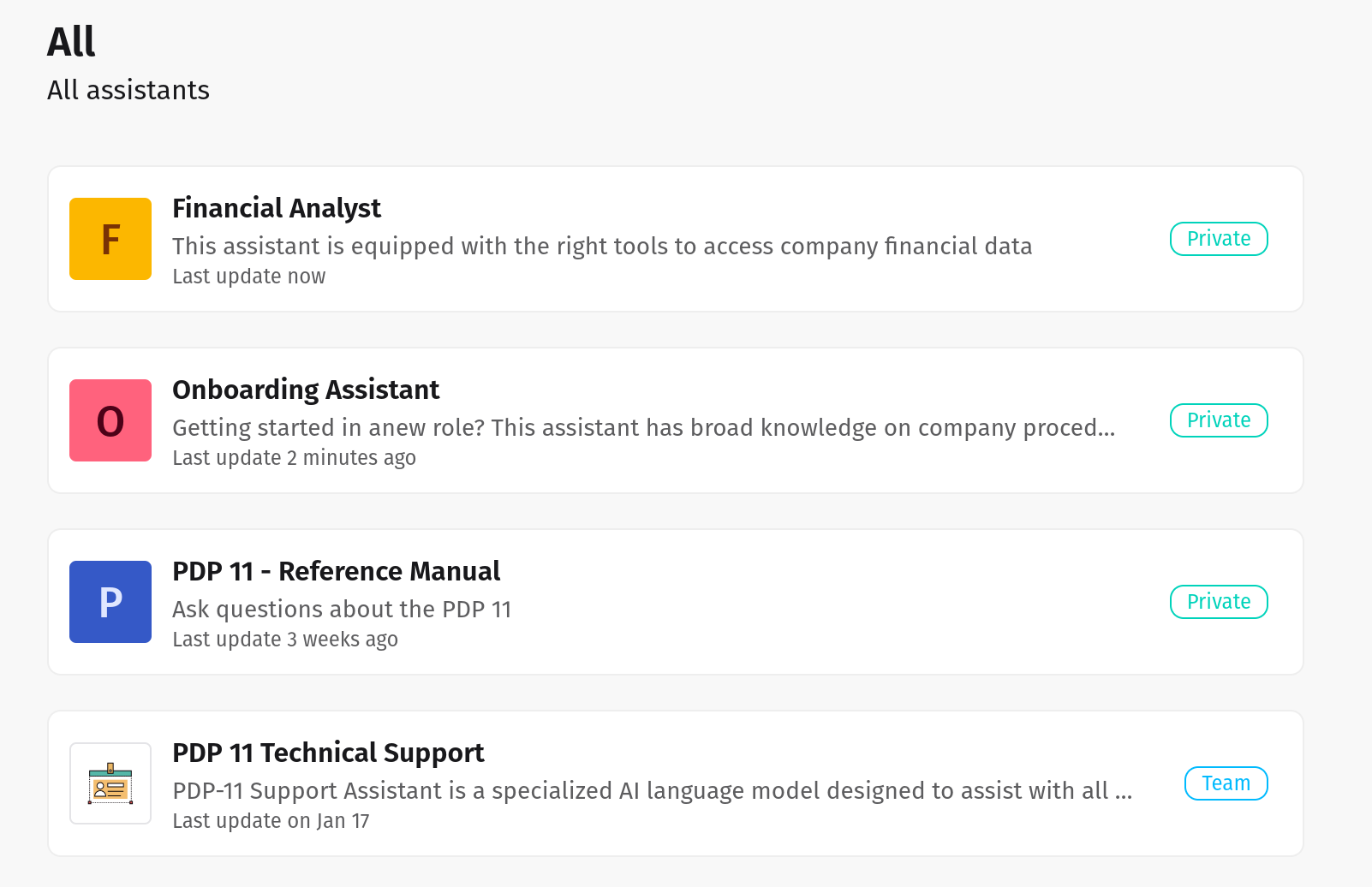
Agentic AI
Create AI Agents in seconds
Use default agents or create new ones tuned to your specific workflows across finance, legal, healthcare, retail, and beyond.
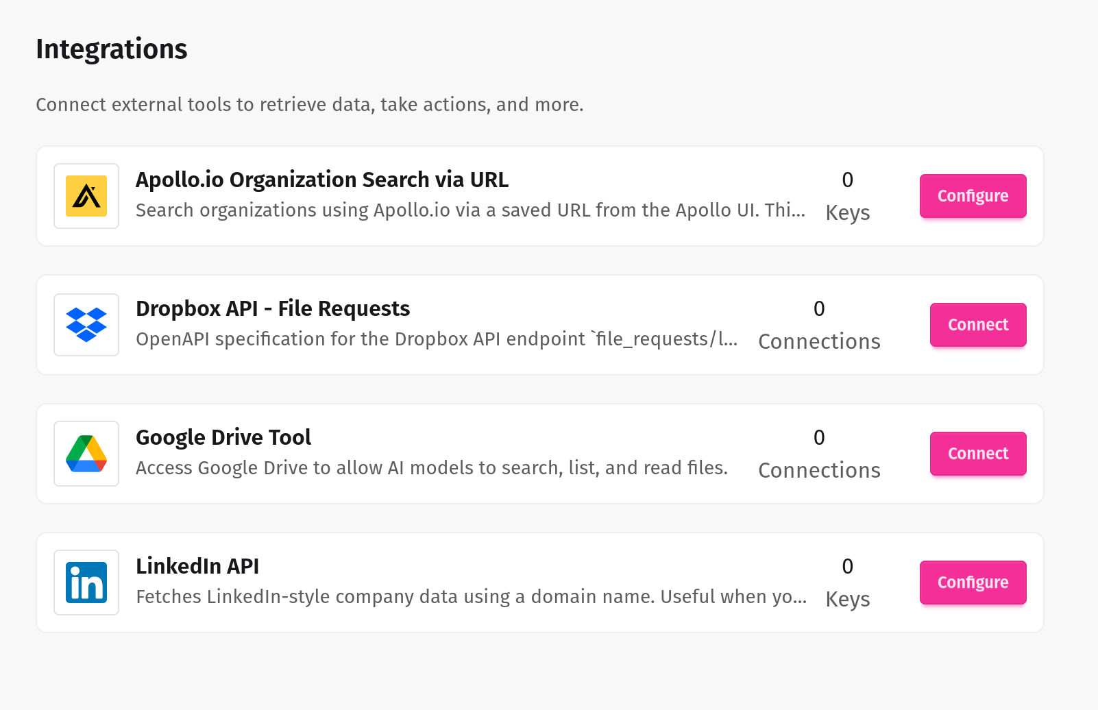
Integrations
Seamlessly connect internal and external systems
Our LLM tools integrate effortlessly with your enterprise systems, ensuring smooth, secure, and intelligent automation across your entire workflow.
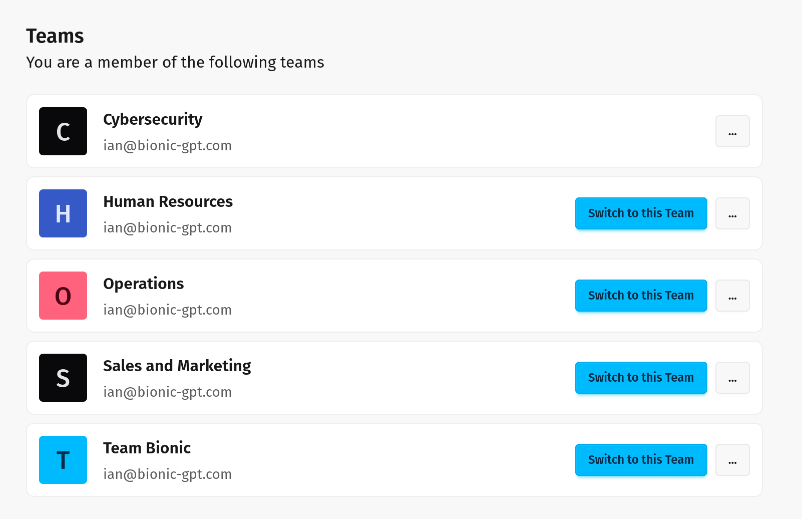
Teams
Seamless Integration for Enhanced Collaboration
Empower your teams with AI that works where they do. Bionic integrates seamlessly into your workflows, providing advanced capabilities without sacrificing security. Your data stays private, enabling trustworthy collaboration and innovation.
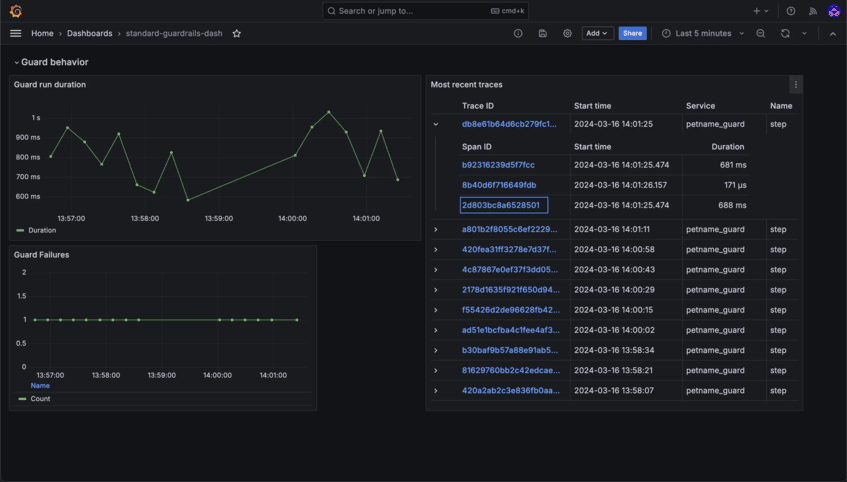
Observability and Auditability
Stay in Control with Detailed Insights
Monitor usage, track interactions, and ensure compliance with robust observability and auditability tools. Transparency and accountability are built right into Bionic.
Bionic Features
A comprehensive solution for all your AI needs.

Agentic Assistants
Connect assistants to your systems and your data.

Team-Based Permissions
Control data access and ensure security by allowing teams to manage permissions.

Full Observability
Gain insights into usage and compliance with detailed dashboards and logs.

Cost Control
Set usage limits by user and team to manage costs effectively.

Advanced Encryption
Ensure data security with encryption at rest, in transit, and during runtime.

Scalable Architecture
Built on Kubernetes for maximum scalability and reliability.
Testimonials
Having the flexibility to use the best model for the job has been a game-changer. Bionic's support for multiple models ensures we can tailor solutions to specific challenges, delivering optimal results every time.
 EmmatData Scientist
Bionic's observability feature, which logs all messages into and out of the models, has been critical for ensuring compliance in our organization. It gives us peace of mind and robust accountability.
 PatrickCompliance Officer
Benefits
AI Your Teams Will Actually Use — and Trust
Accelerate Generative AI Adoption
Boost productivity with a solution that's simple to implement and use securely.
Custom AI Assistants (Agentic RAG)
Utilize your data to create AI assistants that deliver smarter, tailored responses.
Data Compliance and Auditability
Enjoy the advantages of generative AI with robust data governance and compliance.
Frequently asked questions
Bionic runs entirely within your environment, meaning your data never leaves your control. Unlike traditional AI models, there's no need to send information to external servers, eliminating the risk of leaks or unauthorized access.
Yes! Bionic delivers the same advanced AI capabilities as Chat-GPT, with the added advantage of running securely within your infrastructure. You get the full power of GPT without compromising privacy or control.
Absolutely. Bionic allows you to customize and fine-tune the AI using your own data, ensuring it provides accurate, context-aware insights and performs tasks specific to your business requirements.
Bionic includes powerful observability and auditability features. You can track usage, monitor performance, and ensure compliance with detailed logs and insights into how the AI is being used.
Yes. Bionic is designed with security and compliance in mind, making it ideal for industries with strict data protection requirements. It keeps sensitive information private while meeting regulatory standards.
Built with Enterprise Security, Privacy, and Compliance at Its Core
Deploy MCP is designed with enterprise-grade security, privacy, and compliance controls from day one.
Run fully managed in our cloud or deploy on premise to keep sensitive data inside your perimeter.